Neural networks on the Raspberry Pi: More Neurons

A brief introduction to ANNs - part 2

The previous example of a neuron was a bit far-fetched. Its activation function doubled the weighted sum of its inputs. A simpler (and more useful) variant just returns the sum of its weighted inputs. This is known as a linear neuron.

The linear neuron

In APL, you could implement the linear neuron like this:

ln←{+/⍺×⍵}

and use it like this:

1 0.5 1 ln 0.1 1 0.3

0.9

Inner product

However, there's a neater and more idiomatic way to define it in APL. A mathematician would call the ln function the dot product or inner product of ⍺ and ⍵ and in APL you can write it as

ln←{⍺+.×⍵}

There are several reasons to use the inner product notation. It's concise, it's fast to execute, and (as we'll see later) it allows us to handle more than one neuron without having to write looping code.

Linear neurons are sometimes used in real-world applications; another type of neuron you're likely to come across is the perceptron.

The Perceptron

The output of a linear neuron is a real number. The output of a perceptron is binary: a 0 or a 1. This is useful in classification networks, where the output of a perceptron might be used to indicate the presence or absence of a particular feature, An output of zero would mean the feature was absent, while an output of 1 would mean that the feature was present.

Let's look at a concrete application, which we'll come back to later in this series.

An example - handwritten number recognition

Let's imagine that you want to construct a neural network to recognise handwritten digits. The input to your network might be a 28 x 28 matrix of pixels. A matrix of real numbers might represent how bright each pixel is.

You might have ten perceptrons corresponding to the digits 0 to 9. When the image of a handwritten digit is input, the relevant perceptron should fire. In other words, its output should be 1.

The perceptron firing rule

A perceptron calculates its output by looking at the value of the weighted sum of its inputs, just like a linear neuron. However, a perceptron outputs 0 if the sum is zero or negative, and it outputs a 1 if the sum is positive number.

Implementing the Perceptron in APL

You could define the perceptron like this:

p←{0<⍺+.×⍵}

and test it like this:

0.1 1 0.3 p 1 0.5 1

0.1 1 0.3 p 1 0.5 ¯1

0.1 1 0.3 p 1 ¯0.5 ¯1

Notice that you represent negative numbers in APL using' ¯' rather than '-', which means 'do a subtraction'.

The bias input to the perceptron

If you look at a typical article on the perceptron, you will see that the algorithm it gives often includes an extra term called the bias b. Here's the definition from the Wikipedia article:

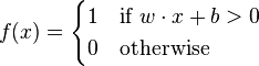
The bias is just like the other inputs except that its contribution is not weighted. To keep your code simple, you can do what many neural networks do. You can treat the bias term as the first element in the input vector, and prefix the weights by the constant 1.

Now when you calculate the inner product of the extended inputs and weights the bias is added to the weighted inputs.

Here's the code:

p2←{0<⍺+.×1,⍵}

In APL the comma (called catenate) is the symbol you use to concatenate two arrays together. In the definition of p2, the 1 is added to the beginning of the vector of weights ⍵. The bias b is the first element of the input vector ⍺.

You can test p2 like this:

0.1 1 0.3 p2 0.5 1

0.1 1 0.3 p2 ¯0.5 ¯1

Here the bias is 0.1 and the other inputs are 1 and 0.3. The weights of the two inputs are 0.5 and 1

Implementing multiple perceptrons

A single perceptron can't do much on it's own. A useful application is likely to have lots of neurons.These are often grouped into layers, and in many cases the layer is fully-connected.

A fully-connected layer of neurons is a collection of neurons in which

each neuron is of the same type
each neuron has its own set of weights
each neuron receives all of the inputs to the layer

The layer has a vector of inputs. The inputs of every neuron are the elements of that vector.

The layer has a vector of outputs. Each element in the output vector is the output from a single neuron.

Using matrices in APL

Since there are multiple neurons, each of which has its own weights, you can represent the weights as a matrix. Column i of the matrix should contain the weights for neuron i.

In APL you can create a matrix by using the reshape function which is represented by the Greek letter rho.

Create a matrix like this:

mat←2 4⍴20

mat

20 20 20 20

You've created a matrix with two rows and four columns. Each entry in the matrix is the number 20.

Creating random test data

You can create test data with a bit more variety like this:

mat←?2 4⍴20

mat

14 11 7 4

10 3 13 15

The ? function (called roll) rolls a 20-sided die for each element in its argument. Your expression created an array of 2 by 4 random numbers.

They are not really random, of course, but they will be different each time you evaluate that expression. So don't be surprised when the values in your version of mat are different from mine!

Even that set of values can be improved on. Try this:

mat←0.1×¯10+?2 4⍴20

mat

0 ¯0.9 0.4 0.6

¯0.4 0.1 ¯0.6 ¯0.9

Remember how APL parses expressions? You can read that first line as 'multiply by 0.1 the result of adding minus ten to a 2 by 4 matrix of numbers in the range 1 to 20'.

The APL is a bit more concise :)

Testing time

Time to try out your layer. Each neuron takes the same vector of inputs. In your case, that vector should have three elements: one for the bias and two for the weights. Create a vector of inputs like this:

inputs ← 0.2 0.3 0.1

See what happens if you try

inputs p2 mat

LENGTH ERROR

p2[0] p2←{0<⍺+.×1,⍵}

∧

Oops! Something has gone wrong. APL's error message has told you the sort of problem it encountered, and what it was executing when the problem occurred.

To understand the source of the problem, try evaluating

1,mat

1 0 ¯0.9 0.4 0.6

1 ¯0.4 0.1 ¯0.6 ¯0.9

Aha! APL has concatenated the 1 at the start of the matrix. That was right when you had a vector argument, but not for a matrix. Try this:

1⍪mat

1 1 1 1

0 ¯0.9 0.4 0.6

¯0.4 0.1 ¯0.6 ¯0.9

That strange comma-with-a-bar means catenate in the last dimension, which will work for vectors and matrices. Change the definition of p2 to be

p2←{0<⍺+.×1⍪⍵}

and run inputs p2 mat again.

It works! With a minor change, you now have code that works equally well for one or many neurons.

That's enough for now. In the next article, we'll look at what the perceptron can and cannot do. We'll also look at other types types of neuron.

Search This Blog

RAREblog