RAREblog

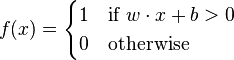
A brief introduction to ANNs - part 3 In the previous post about ANNs we looked at the linear neuron and the perceptron. Perceptrons have been used in neural networks for decades, but they are not the only type of neuron in use today. When they were first invented, they seemed capable of learning almost anything. However, in 1969, Minsky and Papert published their book 'Perceptrons' which showed that a single perceptron could never be trained to perform the XOR function. You'll see in the next post why this is so (and why it's not a huge problem), but for now, let's look at three other common neuron models. Like the linear neuron and perceptron, these start by calculating the weighted sum of their inputs. Recall that you can implement the linear neuron like this:       ln←{⍺+.×⍵} sigmoid neuron calculates the same weighted sum of inputs, but then it applies the sigmoid function to the result. The sigmoid function is defined in wikip...

If you like coding and s olving problems, and are a full-time student , you cou ld win up to $2000 and an expenses-paid trip to a conference in Glasgow later this year. All you need is a computer and some free software. The computer could be a Ras pberry Pi (any model) or a lap top running Windows, O S /X or Lin ux. I' ll tell you where to get th e APL software further down th is post .   First, though, a warning. If you enter this competition it could change your life! I’m serious. Just under f ifty years ago I had a chance to learn APL. I did, and it shaped my whole career. I'm still using A PL to research neural networks . Now, if you want, it’s your turn. The Dyalog APL 2016 problem solving competition   Dyalog have just announced their annual APL problems solving competition. They want to introduce more people to this extraordinary, powerful language. If you are a full time student you could win a big cash prize (up to $2000) and an expenses-paid trip t...

Yesterday saw the arrival of a Raspberry Pi robot kit from T he Pi Hut , and I'm finding it hard not to drop everything and have a play. The Pi Hut has close links with CamJam . CamJam is, I think, the first Raspberry Jam, based in the Cambridge area. Working with The Pi Hut they have created three excellent EduKits: inexpensive, fun kits which introduce Raspberry Pi owners of all owners to the fun of physical computing. The earlier kits came with excellent instructions and the Robot kit does too. I'm sure I will succumb to temptation and start exploring the kit in the next day or two. Expect a progress report soon. My immediate priority is more urgent. I'm talking at the BAA meeting tomorrow, and I need to make sure I'm properly prepared. Dyalog Visit I nearly blew it earlier this week. I went along to visit my friends at Dyalog to talk about my neural network research and show them APL running on the new Pi zero . I thought I had taken everything ...

Spot the difference! The new Raspberry Pi zero is out and it has a camera connector . The picture on the right compares the new zero with its predecessor. They are very, very similar but the clever folks at Pi towers have re-routed the board to make room for a camera connector while keeping the size of the board unchanged. I've had a chance to play with the new Pi for a few days now and I love it. You can read my plans below but the main thing is that the new feature has been added without sacrificing the zero's already awesome capabilities. As you'd expect, existing software runs just as it did before. The new zero is currently in stock at several dealers in the UK and the USA. Details are on the Raspberry Pi website . Dealer info is at the bottom of their post. A camera has been one of the most-requested features for the zero. It opens up a huge range of new, exciting projects. There will be a huge demand for the new zero. Let's hope the stocks hold out ...

A brief introduction to ANNs - part 2 The previous example of a neuron was a bit far-fetched. Its activation function doubled the weighted sum of its inputs. A simpler (and more useful) variant just returns the sum of its weighted inputs. This is known as a linear neuron. The linear neuron In APL, you could implement the linear neuron like this:        ln←{+/⍺×⍵}    and use it like this:        1 0.5 1 ln 0.1 1 0.3 0.9 Inner product However, there's a neater and more idiomatic way to define it in APL. A mathematician would call the ln function the dot product or inner product of ⍺ and ⍵ and in APL you can write it as       ln←{⍺+.×⍵} There are several reasons to use the inner product notation. It's concise, it's fast to execute, and (as we'll see later) it allows us to handle more than one neuron without having to write looping code. Linear neurons are sometimes used in real-...

A brief introduction to ANNs - part 1 ANNs (Artificial Neural Networks) are systems that can process information using connected components called neurons . ANNs are inspired by real (biological) neural networks like the brain. ANNs are widely used for real-world information processing tasks. In the image below (courtesy of Google Street View) you can see that car number plates have been blurred. Google hides them to protect privacy, and the software that recognises what to blur is a Neural Network. Image courtesy Google StreetView The software   As I said yesterday , I developed the software in APL on a Raspberry Pi. You’ll find instructions on how you can run it further down. Neurons An ANN is made up of neurons . Neurons are usually grouped into one or more layers. Many types of neuron have been proposed, but they all have certain characteristics in common. A neuron has one or more inputs and a single output. Associated with each input is a weight....